Focus on the Interest Rate on Reserve Balances
This Page One Economics essay describes the new key tool of monetary policy: the interest rate on reserve balances.
Focus on Large-Scale Asset Purchases
This Page One Economics essay describes the use of temporary open-market operations and large-scale asset purchases to support the flow of credit to households and businesses.
Storytelling with Data and FRED Interactive Modules

Adjusting for Inflation: Learn how to use FRED® to visualize the difference between nominal and real values. The FRED Interactive modules can be embedded in your learning management system.
Quiz Yourself on the New Tools of Monetary Policy
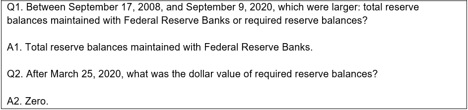
Q1. Between September 17, 2008, and September 9, 2020, which were larger: total reserve balances maintained with Federal Reserve Banks or required reserve balances?
Q2. After March 25, 2020, what was the dollar value of required reserve balances?
Q1. How do overnight repurchase agreements impact financial markets? Do they add or subtract liquidity?
Q2. Between September 2019 and September 2020, when did the value of overnight repurchase agreements peak?
Q1. How do reverse overnight repurchase agreements impact financial markets? Do they add or subtract liquidity?
Q2. Between January 2020 and January 2022, when did the value of reverse overnight repurchase agreements peak?

You can share these graphs with your students using this dashboard. To customize this dashboard, just click the “Save to My Account” button at the top of the dashboard.